


Overview
AlphaLISA™ immunoassay data can be fit to either a linear curve (using just the linear portion of your data) or a dose-response curve. A dose response curve (or sigmoidal or 4PL curve) is typically used to process AlphaLISA immunoassay data in order to take advantage of the full dynamic range of the assay. These types of curves can be fitted using standard statistical software, such as GraphPad Prism® or Microsoft® Excel® with Solver plug-in. For dose-response curves, 1/Y2 weighting should be used for curve fitting. After fitting a standard curve, you can interpolate the concentration of analyte for your unknowns.
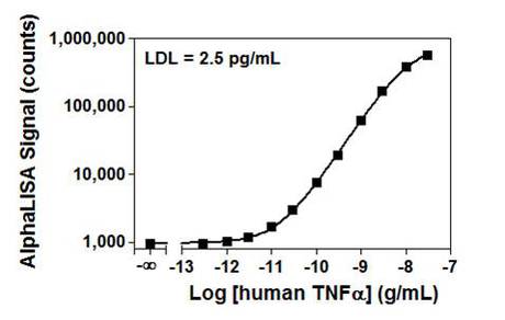
Figure 1. Standard curve for an AlphaLISA TNFα assay. The standard curve was run in AlphaLISA Immunoassay Buffer for these experiments. The data were fit in GraphPad Prism® using a dose-response curve.
Is there any special reason for the 1/Y2 weighting? Data weighting is required because errors are not the same across the curve. If the error was coming mainly from the instrument (e.g. +/- 1,000 counts everywhere), the weighting wouldn’t be required. At the bottom of the curve, values would be 1,000 +/- 1,000 and at the top of the curve, values would be 1,000,000 +/- 1,000. But the error is more a percentage of the signal and is due to sample handling and experimental variation (e.g. X +/- 5%, i.e. 1,000 +/- 50 and 1,000,000 +/- 50,000). In this case, data weighting is recommended.
A residual plot is a good method to determine if the fit is a good one (including data weighting). Residuals are the distance between the curve (fit) and the experimental values. In theory, the residuals should be distributed equally around the mid-point, with equal errors. If they are not at one end of the residual plot, it means the fit is not ideal. For example, see below two curves and the statistical residual plots without and with 1/Y2 for the same set of data.
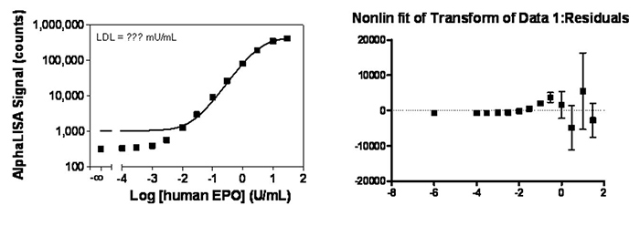
Figure 2. AlphaLISA immunoassay data analysis without weighting.
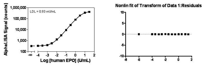
Figure 3. AlphaLISA immunoassay data analysis with weighting.
The hook effect
If your standard curve begins to decrease at the higher concentrations of analyte tested (see Fig. 4), you may be seeing a “hook effect”. The hook effect occurs when you have saturated your beads with analyte. Excess analyte disrupts associations between Donor and Acceptor beads beyond the hook point.
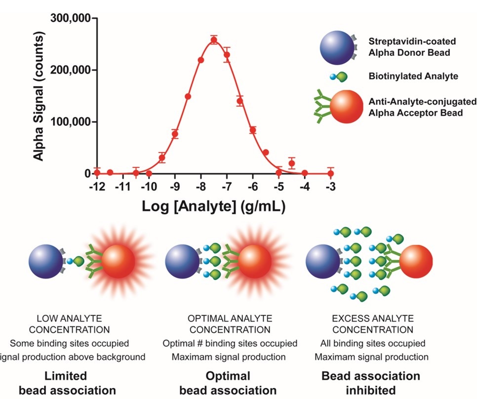
Figure 4. The hook effect. The top graph shows data for an AlphaLISA immunoassay. The signal increases with increasing concentrations of analyte, until you reach the hook point. At this point, the signal begins to decrease with increasing concentrations of analyte. The illustration underneath shows how increasing concentrations of analyte can disrupt interactions between Donor and Acceptor bead when the system is saturated.
If you see a hook effect, simply omit the standards with concentrations beyond the hook point from your data before fitting your standard curve.
Calculating sensitivity (lower detection limit)
Using your standard curve, you can calculate the sensitivity (lower detection limit, LDL) for your assay using the following equation:
LDL = mean (zeroes) + 3 SD
The lower detection limit (LDL or LLD) is equivalent to the concentration interpolated from a signal corresponding to the mean of your “zero analyte” signals + 3 standard deviations.
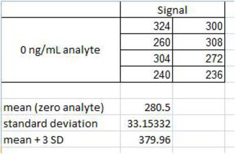
Figure 5. Calculation of mean (zeroes) + 3 SD. The signal from samples corresponding to 0 ng/mL analyte is recorded. The mean (in this case, 280.5) and standard deviation (in this case, 33.15332) are calculated. The value corresponding to the mean plus three standard deviations is calculated (in this case, 379.96). This value (379.96) is used as an "unknown". The concentration of analyte corresponding to this signal is then interpolated from the standard curve (not shown). Calculations in the figures were performed using Microsoft® Excel®.
For research use only. Not for use in diagnostic procedures.
The information provided above is solely for informational and research purposes only. Revvity assumes no liability or responsibility for any injuries, losses, or damages resulting from the use or misuse of the provided information, and Revvity assumes no liability for any outcomes resulting from the use or misuse of any recommendations. The information is provided on an "as is" basis without warranties of any kind. Users are responsible for determining the suitability of any recommendations for the user’s particular research. Any recommendations provided by Revvity should not be considered a substitute for a user’s own professional judgment.